Beginner guide – How to build Spam classifier with Naive Bayes

In this article, I would like to show how a simple algorithm such as naive Bayes can actually produce significant results. I will go through the algorithms in a real dataset and explaining every step in the preprocessing of the text to the pros/cons of the algorithm. Naive Bayes algorithm applies probabilistic computation in a classification task. This algorithm falls under the Supervised Machine Learning algorithm, where we can train a set of data and label them according to their categories.

What we want to achieve

We will be using Naive Bayes to create a model that can classify SMS as spam or not spam (ham) based on the dataset provided. As humans, we can maybe spot some spammy messages and we look closely we can notice that several contains words such as “win”, “Winner”, “cash”, “prize”. Basically, they want to get our attention so we can click on them. As humans, we can also spot other patterns such as weird characters, lots of capital letters.

The goal is to mimic our human ability to spot those messages by using Naive Bayes. It’s a binary classification which means it’s spam or it is not spam.

Overview

The following project was provided by Udacity which offers online courses from Marketing to AI. This article as well as the blog is not sponsored by Udacity. In this blog post, I present a summarised version of the project so check out the jupyter notebook if you would like to have a deep-dive into the explanations and concepts. This project has been broken down into the following steps:

• Step 0: Introduction to the Naive Bayes Theorem
• Step 1.1: Understanding our dataset
• Step 1.2: Data Preprocessing
• Step 2.1: Bag of Words (BoW)
• Step 2.2: Implementing BoW from scratch (available only on the Jupyter Notebook, not in this article)
• Step 2.3: Implementing Bag of Words in scikit-learn
• Step 3.1: Training and testing sets
• Step 3.2: Applying Bag of Words processing to our dataset.
• Step 4.1: Bayes Theorem implementation from scratch
• Step 4.2: Naive Bayes implementation from scratch
• Step 5: Naive Bayes implementation using scikit-learn
• Step 6: Evaluating our model
• Step 7: Conclusion

Step 0: Introduction to the Naive Bayes Theorem

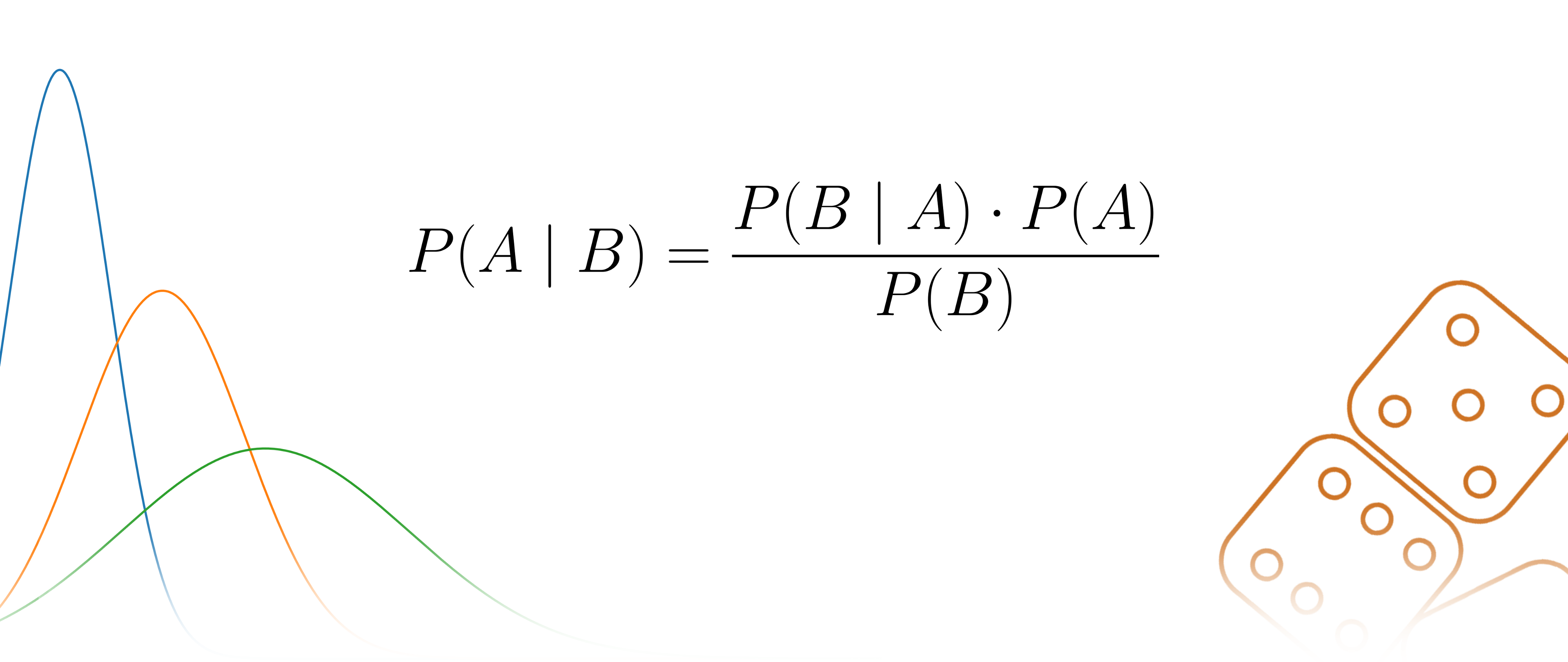
The ‘Naive’ bit of the theorem where it considers each feature to be independent of each other which may not always be the case and hence that can affect the final judgement. In short, Bayes Theorem calculates the probability of a certain event happening (in our case, a message being spam) based on the joint probabilistic distributions of certain other events (in our case, the appearance of certain words in a message).

Step 1.1: Understanding our dataset

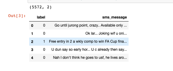
We will be using a dataset originally compiled and posted on the UCI Machine Learning repository which has a very good collection of datasets for experimental research purposes.Here is a preview of the data:
The columns in the data set are currently not named and as you can see, there are 2 columns. The first column takes two values, ‘ham’ which signifies that the message is not spam, and ‘spam’ which signifies that the message is spam.The second column is the text content of the SMS message that is being classified.

Step 1.2: Data Preprocessing

Now that we have a basic understanding of what our dataset looks like, let’s convert our labels to binary variables, 0 to represent ‘ham'(i.e. not spam) and 1 to represent ‘spam’ for ease of computation. Our model would still be able to make predictions if we left our labels as strings but we could have issues later when calculating performance metrics, for example when calculating our precision and recall scores. Hence, to avoid unexpected ‘gotchas’ later, it is good practice to have our categorical values be fed into our model as integers.

df['label'] = df.label.map({'ham':0, 'spam':1})
print(df.shape)
df.head() # returns (rows, columns)

Step 2.1: Bag of Words

What we have here in our data set is a large collection of text data (5,572 rows of data). Most ML algorithms rely on numerical data to be fed into them as input, and email/sms messages are usually text heavy.

Here we’d like to introduce the Bag of Words (BoW) concept which is a term used to specify the problems that have a ‘bag of words’ or a collection of text data that needs to be worked with. The basic idea of BoW is to take a piece of text and count the frequency of the words in that text. It is important to note that the BoW concept treats each word individually and the order in which the words occur does not matter.

Using a process which we will go through now, we can convert a collection of documents to a matrix, with each document being a row and each word (token) being the column, and the corresponding (row, column) values being the frequency of occurrence of each word or token in that document.

For example:

Let’s say we have 4 documents, which are text messages in our case, as follows:

['Hello, how are you!', 'Win money, win from home.', 'Call me now', 'Hello, Call you tomorrow?']

Our objective here is to convert this set of texts to a frequency distribution matrix, as follows:

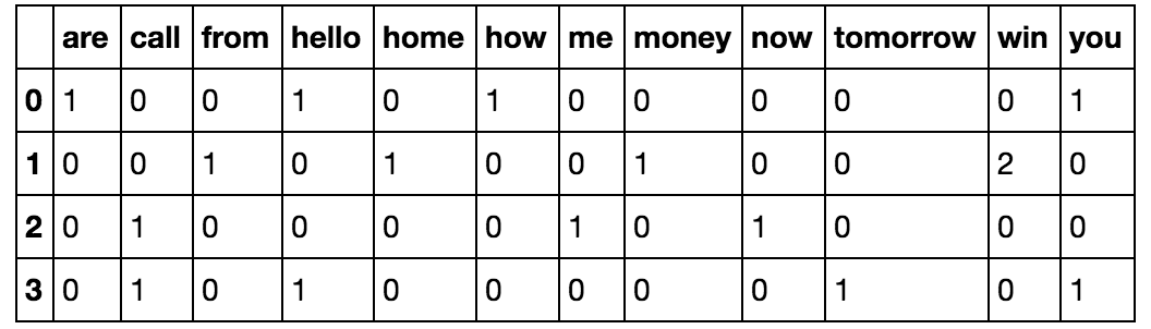
Here as we can see, the documents are numbered in the rows, and each word is a column name, with the corresponding value being the frequency of that word in the document.

Let’s break this down and see how we can do this conversion using a small set of documents.

To handle this, we will be using sklearn’s count vectorizer method which does the following:

• It tokenizes the string (separates the string into individual words) and gives an integer ID to each token.
• It counts the occurrence of each of those tokens.

Step 2.2: Implementing Bag of Words from scratch

(available only on the Jupyter Notebook on my repository, not in this article)

Step 2.3: Implementing Bag of Words in scikit-learn

Here we will look to create a frequency matrix on a smaller document set to make sure we understand how the document-term matrix generation happens. We have created a sample document set ‘documents’.

documents = ['Hello, how are you!',
                'Win money, win from home.',
                'Call me now.',
                'Hello, Call hello you tomorrow?']
from sklearn.feature_extraction.text import CountVectorizer
count_vector = CountVectorizer()

We’re going to use the following parameters that CountVectorizer() offers us

• lowercase = True

  The lowercase parameter has a default value of True which converts all of our text to its lower case form.

• token_pattern = (?u)\\b\\w\\w+\\b

  The token_pattern parameter has a default regular expression value of (?u)\\b\\w\\w+\\b which ignores all punctuation marks and treats them as delimiters, while accepting alphanumeric strings of length greater than or equal to 2, as individual tokens or words.

• stop_words

  The stop_words parameter, if set to english will remove all words from our document set that match a list of English stop words defined in scikit-learn. Considering the small size of our dataset and the fact that we are dealing with SMS messages and not larger text sources like e-mail, we will not use stop words, and we won’t be setting this parameter value.

Result:

['are', 'call', 'from', 'hello', 'home', 'how', 'me', 'money', 'now', 'tomorrow', 'win', 'you']

doc_array = count_vector.transform(documents).toarray()
frequency_matrix = pd.DataFrame(doc_array, 
                                columns = count_vector.get_feature_names())

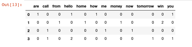
One potential issue that can arise from using this method is that if our dataset of text is extremely large (say if we have a large collection of news articles or email data), there will be certain values that are more common than others simply due to the structure of the language itself. For example, words like ‘is’, ‘the’, ‘an’, pronouns, grammatical constructs, etc., could skew our matrix and affect our analyis. There are a couple of ways to mitigate this. One way is to use the stop_words parameter and set its value to english. This will automatically ignore all the words in our input text that are found in a built-in list of English stop words in scikit-learn. Another way of mitigating this is by using the tfidf method.

Step 3.1: Training and testing sets

Now that we understand how to use the Bag of Words approach, we can return to our original, larger UCI dataset and proceed with our analysis. Our first step is to split our dataset into a training set and a testing set so we can first train, and then test our model.

Now we’re going to split the dataset into a training and testing set using the train_test_split method in sklearn, and print out the number of rows we have in each of our training and testing data. We split the data using the following variables:

• X_train is our training data for the ‘sms_message’ column.
• y_train is our training data for the ‘label’ column
• X_test is our testing data for the ‘sms_message’ column.
• y_test is our testing data for the ‘label’ column.

from sklearn.cross_validation import train_test_split

X_train, X_test, y_train, y_test = train_test_split(df['sms_message'], 
                                                    df['label'], 
                                                    random_state=1)

Step 3.2: Applying Bag of Words processing to our dataset.

• First, we have to fit our training data (X_train) into CountVectorizer() and return the matrix.
• Secondly, we have to transform our testing data (X_test) to return the matrix.

Note that X_train is our training data for the ‘sms_message’ column in our dataset and we will be using this to train our model.

X_test is our testing data for the ‘sms_message’ column and this is the data we will be using (after transformation to a matrix) to make predictions on. We will then compare those predictions with y_test in a later step.

The code for this segment is in 2 parts. First, we are learning a vocabulary dictionary for the training data and then transforming the data into a document-term matrix; secondly, for the testing data we are only transforming the data into a document-term matrix.

# Instantiate the CountVectorizer method
count_vector = CountVectorizer()

# Fit the training data and then return the matrix
training_data = count_vector.fit_transform(X_train)

# Transform testing data and return the matrix. Note we are not fitting the testing data into the CountVectorizer()
testing_data = count_vector.transform(X_test)

Step 4.1: Bayes Theorem implementation from scratch

Now that we have our dataset in the format that we need, we can move onto the next portion of our mission which is the algorithm we will use to make our predictions to classify a message as spam or not spam. Remember that at the start of the mission we briefly discussed the Bayes theorem but now we shall go into a little more detail. In layman’s terms, the Bayes theorem calculates the probability of an event occurring, based on certain other probabilities that are related to the event in question. It is composed of “prior probabilities” – or just “priors.” These “priors” are the probabilities that we are aware of, or that are given to us. And Bayes theorem is also composed of the “posterior probabilities,” or just “posteriors,” which are the probabilities we are looking to compute using the “priors”.

Let us implement the Bayes Theorem from scratch using a simple example. Let’s say we are trying to find the odds of an individual having diabetes, given that he or she was tested for it and got a positive result. In the medical field, such probabilities play a very important role as they often deal with life and death situations.

We assume the following:

P(D) is the probability of a person having Diabetes. Its value is 0.01, or in other words, 1% of the general population has diabetes (disclaimer: these values are assumptions and are not reflective of any actual medical study).

P(Pos) is the probability of getting a positive test result.

P(Neg) is the probability of getting a negative test result.

P(Pos|D) is the probability of getting a positive result on a test done for detecting diabetes, given that you have diabetes. This has a value 0.9. In other words the test is correct 90% of the time. This is also called the Sensitivity or True Positive Rate.

P(Neg|~D) is the probability of getting a negative result on a test done for detecting diabetes, given that you do not have diabetes. This also has a value of 0.9 and is therefore correct, 90% of the time. This is also called the Specificity or True Negative Rate.

The Bayes formula is as follows: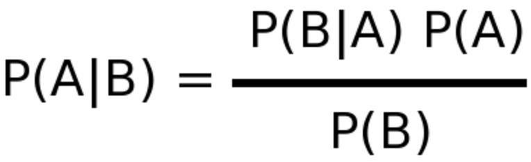

• P(A) is the prior probability of A occurring independently. In our example this is P(D). This value is given to us.

• P(B) is the prior probability of B occurring independently. In our example this is P(Pos).

• P(A|B) is the posterior probability that A occurs given B. In our example this is P(D|Pos). That is, the probability of an individual having diabetes, given that this individual got a positive test result. This is the value that we are looking to calculate.

• P(B|A) is the prior probability of B occurring, given A. In our example this is P(Pos|D). This value is given to us.

Putting our values into the formula for Bayes theorem we get:

P(D|Pos) = P(D) * P(Pos|D) / P(Pos)

The probability of getting a positive test result P(Pos) can be calculated using the Sensitivity and Specificity as follows:

P(Pos) = [P(D) * Sensitivity] + [P(~D) * (1-Specificity))]

# P(D)
p_diabetes = 0.01

# P(~D)
p_no_diabetes = 0.99

# Sensitivity or P(Pos|D)
p_pos_diabetes = 0.9

# Specificity or P(Neg|~D)
p_neg_no_diabetes = 0.9

# P(Pos)
p_pos = (p_diabetes * p_pos_diabetes) + (p_no_diabetes * (1 - p_neg_no_diabetes))
print('The probability of getting a positive test result P(Pos) is: {}',format(p_pos))

´The probability of getting a positive test result P(Pos) is: {} 0.10799999999999998´

Using all of this information we can calculate our posteriors as follows:

The probability of an individual having diabetes, given that, that individual got a positive test result:

P(D|Pos) = (P(D) * Sensitivity)) / P(Pos)

The probability of an individual not having diabetes, given that, that individual got a positive test result:

P(~D|Pos) = (P(~D) * (1-Specificity)) / P(Pos)

The sum of our posteriors will always equal 1.

The formula is: P(D|Pos) = (P(D) * P(Pos|D) / P(Pos)

p_diabetes_pos = (p_diabetes * p_pos_diabetes) / p_pos
print('Probability of an individual having diabetes, given that that individual got a positive test result is:\
',format(p_diabetes_pos))

Probability of an individual having diabetes, given that that individual got a positive test result is: 0.08333333333333336

Compute the probability of an individual not having diabetes, given that, that individual got a positive test result. In other words, compute P(~D|Pos).

The formula is: P(~D|Pos) = P(~D) * P(Pos|~D) / P(Pos)

Note that P(Pos|~D) can be computed as 1 – P(Neg|~D).

Therefore: P(Pos|~D) = p_pos_no_diabetes = 1 – 0.9 = 0.1

# P(Pos/~D)
p_pos_no_diabetes = 0.1

# P(~D|Pos)
p_no_diabetes_pos = (p_no_diabetes * p_pos_no_diabetes) / p_pos
print('Probability of an individual not having diabetes, given that that individual got a positive test result is:'\
,p_no_diabetes_pos)

The analysis shows that even if you get a positive test result, there is only an 8.3% chance that you actually have diabetes and a 91.67% chance that you do not have diabetes. This is of course assuming that only 1% of the entire population has diabetes which is only an assumption.

What does the term ‘Naive’ in ‘Naive Bayes’ mean ?

The term ‘Naive’ in Naive Bayes comes from the fact that the algorithm considers the features that it is using to make the predictions to be independent of each other, which may not always be the case. So in our Diabetes example, we are considering only one feature, that is the test result. Say we added another feature, ‘exercise’. Let’s say this feature has a binary value of 0 and 1, where the former signifies that the individual exercises less than or equal to 2 days a week and the latter signifies that the individual exercises greater than or equal to 3 days a week. If we had to use both of these features, namely the test result and the value of the ‘exercise’ feature, to compute our final probabilities, Bayes’ theorem would fail. Naive Bayes’ is an extension of Bayes’ theorem that assumes that all the features are independent of each other.

Step 4.2: Naive Bayes implementation from scratch

Let’s say that we have two political parties’ candidates, ‘Jill Stein’ of the Green Party and ‘Gary Johnson’ of the Libertarian Party and we have the probabilities of each of these candidates saying the words ‘freedom’, ‘immigration’ and ‘environment’ when they give a speech:

• Probability that Jill Stein says ‘freedom’: 0.1 ———> P(F|J)

• Probability that Jill Stein says ‘immigration’: 0.1 —–> P(I|J)

• Probability that Jill Stein says ‘environment’: 0.8 —–> P(E|J)

• Probability that Gary Johnson says ‘freedom’: 0.7 ——-> P(F|G)

• Probability that Gary Johnson says ‘immigration’: 0.2 —> P(I|G)

• Probability that Gary Johnson says ‘environment’: 0.1 —> P(E|G)

And let us also assume that the probability of Jill Stein giving a speech, P(J) is 0.5 and the same for Gary Johnson, P(G) = 0.5.

Given this, what if we had to find the probabilities of Jill Stein saying the words ‘freedom’ and ‘immigration’? This is where the Naive Bayes’ theorem comes into play as we are considering two features, ‘freedom’ and ‘immigration’.

Now we are at a place where we can define the formula for the Naive Bayes’ theorem:

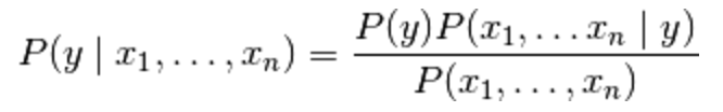
Here, y is the class variable (in our case the name of the candidate) and x1 through xn are the feature vectors (in our case the individual words). The theorem makes the assumption that each of the feature vectors or words (xi) are independent of each other. Applying this to our problem of classifying messages as spam, the Naive Bayes algorithm looks at each word individually and not as associated entities with any kind of link between them. In the case of spam detectors, this usually works, as there are certain red flag words in an email which are highly reliable in classifying it as spam. For example, emails with words like ‘viagra’ are usually classified as spam.

To break this down, we have to compute the following posterior probabilities:

• P(J|F,I): Given the words ‘freedom’ and ‘immigration’ were said, what’s the probability they were said by Jill?

  Using the formula and our knowledge of Bayes’ theorem, we can compute this as follows: P(J|F,I) = (P(J) * P(F|J) * P(I|J)) / P(F,I). Here P(F,I) is the probability of the words ‘freedom’ and ‘immigration’ being said in a speech.

• P(G|F,I): Given the words ‘freedom’ and ‘immigration’ were said, what’s the probability they were said by Gary?

  Using the formula, we can compute this as follows: P(G|F,I) = (P(G) * P(F|G) * P(I|G)) / P(F,I)

Now that you have understood the ins and outs of Bayes Theorem, we will extend it to consider cases where we have more than one feature.

Step 5: Naive Bayes implementation using scikit-learn

We will be using sklearn’s sklearn.naive_bayes method to make predictions on our SMS messages dataset.

Specifically, we will be using the multinomial Naive Bayes algorithm. This particular classifier is suitable for classification with discrete features (such as in our case, word counts for text classification). It takes in integer word counts as its input. On the other hand, Gaussian Naive Bayes is better suited for continuous data as it assumes that the input data has a Gaussian (normal) distribution.

from sklearn.naive_bayes import MultinomialNB
naive_bayes = MultinomialNB()
naive_bayes.fit(training_data, y_train)

Result

MultinomialNB(alpha=1.0, class_prior=None, fit_prior=True)

Now that our algorithm has been trained using the training data set we can now make some predictions on the test data stored in ‘testing_data’ using predict()

predictions = naive_bayes.predict(testing_data)

Step 6: Evaluating our model

Now that we have made predictions on our test set, our next goal is to evaluate how well our model is doing. There are various mechanisms for doing so, so first let’s review them.

Accuracy measures how often the classifier makes the correct prediction. It’s the ratio of the number of correct predictions to the total number of predictions (the number of test data points).

Precision tells us what proportion of messages we classified as spam, actually were spam. It is a ratio of true positives (words classified as spam, and which actually are spam) to all positives (all words classified as spam, regardless of whether that was the correct classification). In other words, precision is the ratio of

[True Positives/(True Positives + False Positives)]

Recall (sensitivity) tells us what proportion of messages that actually were spam were classified by us as spam. It is a ratio of true positives (words classified as spam, and which actually are spam) to all the words that were actually spam. In other words, recall is the ratio of

[True Positives/(True Positives + False Negatives)]

For classification problems that are skewed in their classification distributions like in our case – for example if we had 100 text messages and only 2 were spam and the other 98 weren’t – accuracy by itself is not a very good metric. We could classify 90 messages as not spam (including the 2 that were spam but we classify them as not spam, hence they would be false negatives) and 10 as spam (all 10 false positives) and still get a reasonably good accuracy score. For such cases, precision and recall come in very handy. These two metrics can be combined to get the F1 score, which is the weighted average of the precision and recall scores. This score can range from 0 to 1, with 1 being the best possible F1 score.

We will be using all 4 of these metrics to make sure our model does well. For all 4 metrics whose values can range from 0 to 1, having a score as close to 1 as possible is a good indicator of how well our model is doing.

from sklearn.metrics import accuracy_score, precision_score, recall_score, f1_score
print('Accuracy score: ', format(accuracy_score(y_test, predictions)))
print('Precision score: ', format(precision_score(y_test, predictions)))
print('Recall score: ', format(recall_score(y_test, predictions)))
print('F1 score: ', format(f1_score(y_test, predictions)))

Accuracy score:  0.9885139985642498
Precision score:  0.9720670391061452
Recall score:  0.9405405405405406
F1 score:  0.9560439560439562

Step 7: Conclusion

One of the major advantages that Naive Bayes has over other classification algorithms is its ability to handle an extremely large number of features. In our case, each word is treated as a feature and there are thousands of different words. Also, it performs well even with the presence of irrelevant features and is relatively unaffected by them. The other major advantage it has is its relative simplicity. Naive Bayes’ works well right out of the box and tuning its parameters is rarely ever necessary, except usually in cases where the distribution of the data is known. It rarely ever overfits the data. Another important advantage is that its model training and prediction times are very fast for the amount of data it can handle. All in all, Naive Bayes’ really is a gem of an algorithm!

I also believe that Naive Bayes is very useful even if you’re more advanced. Simple models such as this can be used as baseline for more advanced models. So why not?

Happy coding!